Download data

In this section, you will learn how to order Landsat data from the USGS, including how to search only for the area we are interested in.

You will attempt to find one clear scene (cloud-free or nearly so) per year, over the longest time period available. This must include the period 1987 to 2000, as this will directly be used in the modelling. Any other years that you process could be used to provide a context to growth outside of the target years.

You will then learn how to download the datasets.

Finally, we present one manual and one automated method for scaling the data, subsetting and producing a mask.

You must demonstrate that you have been through all of these steps, providing e.g. email and file link evidence for the files you order from USGS, and demonstrate images in your report (under Method) showing the full scenes and subsets (perhaps as false or real colour composites). You should also show the associated mask files in your report.

You do not need to use the ‘automated’ subsetting method: you can do everything manually if you wish.

If you use the automated method, make sure you provide evidence that you have processed one scene with the manual method (appropriate images/stats at each stage)

Downloading and visualisation tools

The first task is to download the data that you will need.

There are several tools available to you for browsing and ordering Landsat data. See the USGS for a full description of the data products and where to order them.

The area we are interested in is shown below (UTM Zone 49 UL 767385 2533665, LR 827985 2493765):

around the city of Shenzhen:

which is contained in Landsat WRS2 Path 122, Row 44.

You will see that this region is in the bottom right section of the landsat scene:

Use the Surface Reflectance product

For this work, we suggest that you use the surface reflectance products. Ordering these data involves using the USGS Earth Resources Observation and Science (EROS) Center Science Processing Architecture (ESPA) On Demand Interface.

Whilst there are several ways you can select scenes for download, one of the more straightforward is simply to select and order the scenes using EarthExplorer.

See Product Guide: Landsat CDR Surface Reflectance, on-demand version for more details on the products.

There are of course various alternatives to using the surface reflectance product, but one big advantage of using reflectance should be that the spectral and temporal signatures we see in the data are more easily interpreted than using raw Digital Number (DN). Further, this new Landsat product contains quality flags and masks for cloud and other features. The one downside of the current version of the product os that it does not contain thermal the IR band from Landsat.

If you can justify your decision in the write-up, you can choose any of the landsat products available. The notes below however proceed assuming you are using the reflectance data.

Register the first time

The first time you visit the ordering service, you will need to register for an account. Make sure you remember the usename and password you used for registration!

Order Scenes

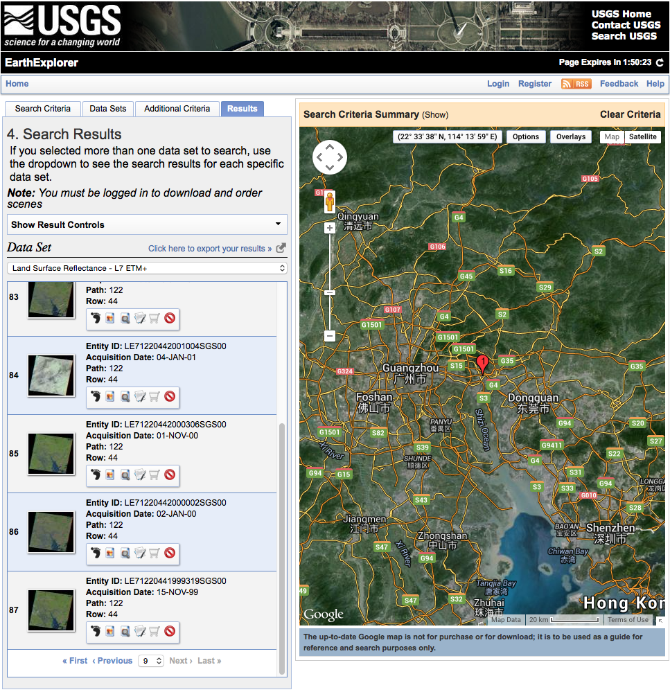
Visit the USGS EarthExplorer site, and search for suitable datasets.

You are looking for datasets for Path 122, Row 44 in the WRS2

and may wish to refine the search criteria (e.g. try only searching for data in January and December). You should consider why it might be appropriate to try to select datasets at the same time of year.

then select one or more of the Landsat sensors in the Landsat CDR option:

Under the tab Additional Criteria, you can force the search to be only for Path 122, Row 44, and e.g. refine the ‘cloud cover’ conditions (e.g. less than 10% might be a place to start).

Note that if you don’t get a suitable set of images for this snalysis, you may have to refine your search conditions (e.g. consider more months).

You now need to look through the results to find scenes approximately 1 year apart for as many years as you can from the archive. You should avoid scenes that have cloud cover in the lower right quadrant of the scene: select only those that appear to be cloud-free.

When you have selected suitable scenes, login to the usgs site (if not already logged in) and add the images you want to the ‘basket’.

You should then check what you have ordered, proceed to ‘checkout’ and order the data.

Since these data are through an ‘on demand’ service, the system will send you an email (to the account you registered) once the datasets are prepared.

Download Scenes

You will be sent an email from the USGS.

You must keep this email to show evidence that you have ordered the data.

The email will give you a web address that will look something like http://espa.cr.usgs.gov/ordering/status/f.bloggs@nasa.gov.

If you have recent or active orders, this web page should show you the status for each file (wait until it says ‘complete’).

Then, you can download the file (using the Download link).

You must keep a record of the download links to show evidence that you have ordered the data, e.g.:

http://espa.cr.usgs.gov/orders/f.bloggs@nasa.gov-0101502242983/LE71220442000306-SC20150224104838.tar.gz

Save all of the download links in a file toi include in your report.

The filename will be something like:

LE71220441999255-SC20150217105511.tar.gz

There is no need to ‘unzip’ or ‘untar’ the file: just download it for the moment.

Make sure you remember which directory you have downloaded the data to.

You should probably download the datasets to you DATA disk, or you might run out of quota, or at least move the files to the DATA disk soon after.

As the files are quite large, it may take some minutes to download each scene.

Subsetting Scenes: Hard

Uncompress a test dataset

The Landsat image scenes contain data over a much greater extent than we need for this practical, and since the datasets are archived (at USGS) there is no need to keep the original files once we have extracted the area we want from them.

In this exercise, we want you to understand how to use the tool ENVI to do some basic operations on image datasets.

As we shall see, it is often easier to write some computer code that will do some automated task over many datasets, but first lets do it the ‘hard’ way (using ENVI).

First, choose one of the Landsat datasets you have downloaded.

In a unix terminal, change directory to where the downloaded files are, e.g.:

%%bash
# NB - don't type 'bash' as above if you are using a unix shell
# The file name may or may not have a .gz on the end

# here, we suppose the download directory to be called 'download'
cd download

# un'tar' (like unzip) the file
tar xvzf LE71220442000306-SC20150224104838.tar

Package the dataset

The file we downloaded contains a set of tif format files (geotiff).

The meaning of the various files is explained in the Product Guide: Landsat CDR Surface Reflectance, on-demand version.

We are primarily interested in the files:

sr_cfmask:

and the files:

sr_band[1-7].

In ENVI, open up all of the sr_cfmask and sr_bandX datasets:

Then select New File Builder from the Raster Management section of the toolbox:

This should allow you to stack the reflectance data from the tif files into a single image dataset.

This in turn should allow you to display, e.g. a false colour composite:

Build a mask

Since the dataset we are using may have some clouds, we should build a mask to identify these areas and not include them in the (land cover) classification.

Select the toolbox option Raster Management -> Masking -> Build Mask, and load the _cmask.tif dataset.

From the table above, we see that we want to not mask pixels with values 0 (clear). If we believe the water mask to be reliable, we could directly use that to represent pixels with the class ‘water’, but for now, let’s assume we need to build out own classification of water pixels. So, allowing ‘clear’ or water pixxels is what we want.

Check Options -> Selected Areas "OFF" (so we are defining which areas not to mask).

You can then clear any masks that might have been defined as you started the tool, then enter 0 and 1 as the Data Min Value and Data Max Value respectively under Options -> Import Data Range:

Then select an output filename (write down what it is … perhaps call it test_mask or similar) and run the masking. This should create an image which has value 1 for areas we don’t want to include and 0 for those we do.

Assuming you have the dataset image loaded and now the mask loaded, you should be able to visualise the impact of the mask, using the ‘transparency’ option, for example. For some cases, you might find the mask is over zealous, and may choose to ignore the mask. If you do so, make sure you document this as part of your ‘method’ section. Provde evidence for the choices you make (e.g. images or statistics to back up a point).

Extract Area of Interest

Under Toolbox -> Raster Management -> Resize Data, select the test data file and, in the box marked Spatial Subset, select the following:

for the minimum and maximum lines and samples.

Continue with the Resize Data ... option, perhaps calling the output file LE71220442000306SGS00_sub or something similar.

Do the same (subsetting) for the mask image (if you intend using it) and name the file something sensible (e.g. LE71220442000306SGS00_sub_mask).

If this has worked properly, you should have only the part of the image we wanted:

Apply Gain Setting

You may find it of use to apply the gain setting of 0.0001 noted in the product data table. You can do this using Toolbox -> Radiometric Correction -> Apply Gain and Offset, setting all of ther gain values to 0.0001 in the list. You might save this as e.g. LE71220442000306SGS00_sub_refl.

Once you have the _sub_refl and _sub_mask files, along with their ancilliary files _sub_refl.enp, _sub_mask.enp and _sub_refl.hdr, _sub_mask.hdr, you should copy these to a new data directory, as these are the files you will work on for the rest of the project.

If you are short of space, you can delete the other files generated.

Subsetting Scenes: Easy

The process you have been through above is instructive when learning the steps you might need to go through in preparing your data, but it is tedious (and unreliable) to do all of this ‘by hand’ for more than a few images.

Another approach is to write a computer program to achieve the same thing.

In fact, this can be directly interfaced with ENVI if you use the programming language `IDL <http://www.exelisvis.co.uk/ProductsServices/IDL.aspx>`__, though some consider the language rather inelegant. For this reason, we will use some codes written in the Python language.

It is not at all vital that you follow the details of the code, though you might find it interesting to try to work out what is going on.

First, we uncompress the files (which files, is controlled by the dirname variable below:

# Uncompress files
%matplotlib inline
import sys
from glob import glob
sys.path.insert(0,'python')
from uncompress_ls import uncompress_ls
from sort_landsat import sort_landsat

# this is where you specify the names of your downloaded files
allofiles = []
for dirname in glob('files/new/LT51220441995364-*.tar.gz'):
    files = uncompress_ls(dirname,temp_dir='temp')
    ofiles = sort_landsat(files)
    allofiles.append(allofiles)
# The list files now contains the temporary
# filenames of the files we uncompressed
# we will delete these at the emd

So these are the files created:

print (allofiles)

[]

Data Visualisation

Now you have one or more datasets of the area, load them into ENVI and explore the data. Provide examples of e.g. interesting spectral profiles, transects, histograms or scatter plots that you would normally produce as part of a data exploration exercise.